GT New Horizons · Ultimate Voltage (UV)
Quantum Computer
The Quantum Computer (QC) is a UV tier multiblock that generates computation through quantum mechanics for the Research Station and a few other multiblocks. It is first required when crafting the UHV mainframe data stick, but remains an integral part of progression up through UXV. There are a few things that must be understood before operating one because careless operation of such a complex machine WILL result in the unintentional destruction of expensive components, and possibly a catastrophic explosion!
Computation is nothing more than an integer input for certain recipes--much like EU. There may exist a minimum throughput requirement, a threshold to reach, or both (NEI tells you everything). Computation is generated every second by the QC, transmitted out through an optical transmission connector, received by an optical reception connector, and "consumed" by the machine or process that needs it. There is no storing computation and there can only be ONE transmission or reception hatch connected to the same optical fiber cables at a time. If absolutely necessary, the Network Switch with QoS can split/join connections but know that it takes both power and maintenance to run.
Script: QC Calculator
Construction
Much like an Assembly Line, the Quantum Computer is built as a series of slices. The first and last slice are the only valid locations for buses/hatches while those in between are primarily for computer racks. Multi-Amp and laser energy hatches are supported. Use the Multiblock Structure Hologram Projector to visualize/build the structure where the projector stack size determines the length.
Unique to the QC is the uncertainty resolver (for maintenance) and the optical transmission connector (for sending computation). There can even be an optical reception connector to add the computation from another QC to its own output (daisy-chaining). All optical hatches are connected with colored optical fiber cable.
Base Structure
- Controller: Front left, 2nd layer
- 6-17 Computer Casing
- 10 Advanced Computer Casing
- 6 Computer Heat Vent
- 2 Computer Rack: Any advanced computer casing, except the outer ones
- 1 Uncertainty Resolver: Any computer casing on the first or last slice
- 1+ Optical Transmission Connector: Any computer casing on the first or last slice
- 0+ Optical Reception Connector: Any computer casing on the first or last slice
- 1+ Energy Hatch: Any computer casing on the first or last slice
- 1 Maintenance Hatch: Any computer casing on the first or last slice
- Mandatory Air: In front of each computer heat vent
Each Additional Slice
- 2 Computer Casing
- 2 Advanced Computer Casing
- 2 Computer Heat Vent
- 2 Computer Rack: Any advanced computer casing, except the outer ones
-
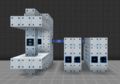 Research Station with two QCs chained together via Optical Fiber Cables.
-
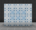
 Left side of the Quantum Computer. The minimum length only supports two computer racks.
-
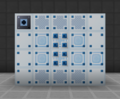
 Right side of the Quantum Computer. No racks or vents.
-
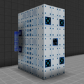 Wallshared and Daisy-Chained QCs.
Wallsharing
QCs may wallshare each of their sides to save on casings and buses/hatches. That includes the uncertainty resolver which can help reduce the time and effort of solving those puzzles. However, do NOT share the optical transmission connector because the computation will neither be reliable nor accurate.
Overclock and Overvolt
In the GUI of the controller, there are two configurable parameters, overclock and overvolt, that change how computation and heat are generated. Higher overclock values contribute the most to computation and higher overvolt values contribute the most to heat. Alone, this would encourage the player to make overclock as high as possible and overvolt as low as possible, but there is a penalty to computation for large differences between these two parameters. Furthermore, overvolt values <1 cause the QC to randomly drop computation proportional to its distance from 1. It is highly encouraged to play around with these parameters, as all the best setups do. See the section on Computer Racks below for more information.
Uncertainty Resolver
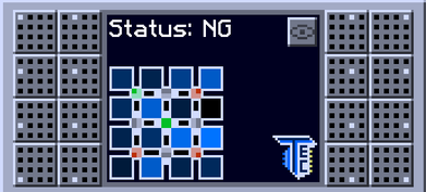
The Quantum Computer has a unique maintenance requirement that can only be fixed by balancing the Schrödinger Matrix inside an uncertainty resolver. This is required for the machine to operate even if there are no other maintenance issues. The interface has the Schrödinger-Matrix in the middle and two sets of 8 buttons on the left and right. Clicking on one button and then another swaps the states (shade/color) of the two corresponding cells in the matrix. The goal of the puzzle is to turn each of the glowing LED lights green by balancing the cells within their measurable area symmetrically around them.
Look closely and you will notice that each LED consists of four pixels with 1-4 of them shaded a slightly darker color. Those darker pixels signify which part of the matrix the LED is measuring, such as the 4 cells in the top left corner or the 8 cells on the right. Use the following images as reference.
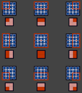 |
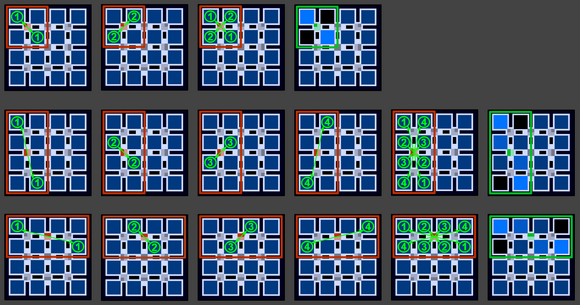 |
Once you identify the measurable area for each LED, start moving any same-color or similar number cells to opposite ends from one another to balance them around the LED. Think of the area as a plate, the LED as a stick holding it up in the air, and the cell colors as weights. Similar weights need to be on opposite ends of the plate to keep the whole thing from falling off the stick. Once all the "plates" are perfectly balanced, the LED lights should turn green and the puzzle is solved. There is a fair amount of tolerance so clicking random buttons actually works surprisingly well, but that's no fun.
The number of LED lights increases with the length of the QC to make the puzzle slightly more challenging, as seen in the following image. The mode refers to the five possible LED configurations and the numbers are the cells that should have the same or at least very similar states. As time passes, the states converge to the same color (50) which automatically solves the puzzle for the player. However, that can be slightly problematic at first because it could cause an odd number of bright cells or one really high number, for example.
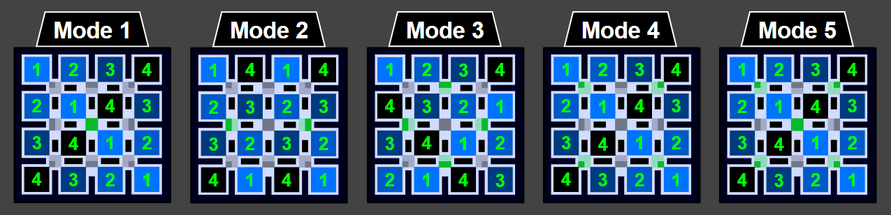
There are two tiers of uncertainty resolvers. The first is the uncertainty resolver X which uses a static shade/color for the states of cells. The second is the uncertainty resolution (UIV) which is perfectly balanced at all times. Again, these hatches can and should be wallshared by multiple QC.
Computer Rack
The QC has 2-24 computer racks depending on the length of the machine. Each rack has four total slots for either circuits (to generate heat and computation) or vents (to dissipate heat). Although conceptually similar to a Nuclear Reactor, the location of the components inside does not matter at all. Every rack is also completely independent from every other rack which means it is not possible to have one rack with all circuits and another with all vents. It is highly recommended to use the exact same setup for every rack.
The COMPUTATION of a rack is the sum of all the computations of the components within. For example, two APU (Tier 3) and two Cooling Cores have 240 + 240 + 0 + 0 = 480 base computation per second. However, computation changes significantly with the values for overclock and overvolt as seen in the equation above.
The HEAT of a rack is a value between 0 and 10,000 and is reported in the interface of the QC or by using a Portable Scanner on the rack. Every component has a certain heat limit which if exceeded will void that component. Breaking or wrenching a rack while it is hot (>2000) or while the QC is actively running similarly voids the components inside. The QC explodes if the heat exceeds 10,000 but no component has a heat limit greater than that, so don't worry too much about ruining your base. Every component also has a heat constant which is proportional to the amount of heat added to the rack every second. Unfortunately, it is not easy to predict where the heat will converge without the script linked at the top so either use that to verify the safety of a particular setup, or use one of the stable setups in the following section.
The POWER CONSUMPTION of a rack is 1A ZPM regardless of the components inside. This is in addition to the 1A ZPM of the QC itself. However, these EU/t values are directly proportional to overclock and overvolt which should increase as the player unlocks better circuits. Be sure to turn on the QC before the research station and only when necessary. Try attaching a wireless item detector cover to the object holder of the research station and have that enable the Quantum Computer(s) via an advanced redstone receiver (internal).
|
| |||||||||||||||||||||||||||||||||||||||||||||||||||||||||||||||||||||||||||||||||||||||||||||||||||||||||||||||||||||||||||||||||||||||||||||||||||||||||||||||||||
Summary
Despite all these numbers and equations, the QC is actually surprisingly simple to use. Here is a quick summary to help you get started.
- Build the QC with the Multiblock Structure Hologram Projector. Add racks, an uncertainty resolver, and an optical transmission connector.
- Repair any maintenance issues and balance the Schrödinger Matrix inside the uncertainty resolver.
- Place circuits and vents inside the racks--probably one of the optimized setups below.
- Adjust the overclock and overvolt values inside the GUI of the controller to increase computation at the cost of power (optional).
- Enable the QC to start sending computation out the optical transmission connector.
Stable Setups
Here are several combinations of circuits and vents for maximizing computation depending on your available resources and progression. The computation and power is per 24 racks or a max length QC. Do not be alarmed if the heat increases rapidly at first--these are designed to converge just below the heat limit of the components. For non-mainframe circuits, use the calculator linked at the top.
| Component 1 | Component 2 | Component 3 | Component 4 | Overclock | Overvolt | Amps (UV) | Computation |
| Crystal Mainframe | Cooling Core | Cooling Core | Cooling Core | 1.73 | 1.41 | 15.25 | 10,416 /s |
| Crystal Mainframe | Crystal Mainframe | Cooling Core | Cooling Core | 1.21 | 1.00 | 7.56 | 13,584 /s |
| APU (Tier 3) | Cooling Core | Cooling Core | Cooling Core | 1.86 | 1.52 | 17.67 | 23,016 /s |
| APU (Tier 3) | APU (Tier 3) | Cooling Core | Cooling Core | 1.43 | 1.03 | 9.21 | 30,216 /s |
| Wetware Mainframe | Cooling Core | Cooling Core | Cooling Core | 2.15 | 1.87 | 25.13 | 27,528 /s |
| Wetware Mainframe | Wetware Mainframe | Cooling Core | Cooling Core | 1.63 | 1.26 | 12.84 | 33,960 /s |
| Bioware Mainframe | Cooling Core | Cooling Core | Cooling Core | 2.63 | 2.35 | 38.63 | 45,792 /s |
| Bioware Mainframe | Bioware Mainframe | Cooling Core | Cooling Core | 1.91 | 1.61 | 19.22 | 53,208 /s |
| Optical Mainframe | Cooling Core | Cooling Core | Cooling Core | 3.20 | 3.00 | 60.00 | 67,416 /s |
| Optical Mainframe | Optical Mainframe | Cooling Core | Cooling Core | 2.35 | 2.04 | 29.96 | 74,256 /s |
| Pico Circuit | Cooling Core | Cooling Core | Cooling Core | 3.95 | 3.80 | 93.81 | 101,304 /s |
| Pico Circuit | Pico Circuit | Cooling Core | Cooling Core | 2.86 | 2.60 | 46.47 | 107,304 /s |
| Quantum Circuit | Cooling Core | Cooling Core | Cooling Core | 4.26 | 4.12 | 109.69 | 144,216 /s |
| Quantum Circuit | Quantum Circuit | Cooling Core | Cooling Core | 3.05 | 2.83 | 53.95 | 150,936 /s |
| Planck Circuit | Cooling Core | Cooling Core | Cooling Core | 4.59 | 4.44 | 127.37 | 186,456 /s |
| Planck Circuit | Planck Circuit | Cooling Core | Cooling Core | 3.27 | 3.06 | 62.54 | 193,512 /s |
Inserting Components
Eventually longer and additional QCs are needed to support the Research Station. At that point it starts to become difficult or annoying to insert components into racks by hand. The following is a simple scalable solution for automatically filling any number of QCs simultaneously. The Ring of Loki is not technically necessary but highly recommended because it greatly expedites the process.
An alternative to the following is building a template QC for copy-pasting with the Matter Manipulator. Do not enable the template QC because the components do not carry over while the machine is running or is too hot.
Method 1: EnderIO
The core mechanic behind this approach is using EnderIO conduits with a speed downgrade to insert one item at a time into the computer racks in a round-robin manner. This approach takes a little bit of time to initially setup but scales to any number of QCs. The only prerequisite is a conduit probe.
| STEP 1 | |
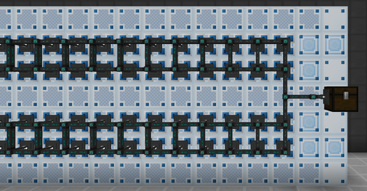
| Connect all computer racks to the same EnderIO conduit network. This can extend to any number of racks, but they must all be chunkloaded.
Use the Ring of Loki and a conduit probe to quickly set every conduit interface to INSERT. Connect a storage chest to the conduit network that contains exactly the required number of rack components. This can also be an ME chest if larger storage is necessary. |
|
| STEP 2 | |
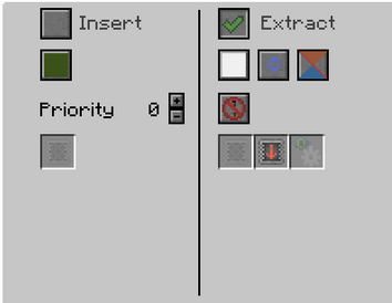
| For the conduit connected to the storage chest, set the mode to EXTRACT, enable ROUND-ROBIN, and insert a SPEED DOWNGRADE. The speed downgrade is necessary because item conduits extract four items at a time by default.
Once ready, set the redstone mode to ALWAYS ACTIVE and wait patiently until the racks are filled. Remove the conduits once complete. |
|